Memory profiling (PyTorch edition)

In this blog, we will explore the usage of the memory by the GPU within a PyTorch framework. We will provide an example of DCGAN and will explore the memory usage of the model during training.

Introduction

Let's consider a simple example of simple model training.

import torch
import torch.nn as nn
import torch.optim as optim
from torchvision import datasets, transforms

########################################################################
# 0.  CONFIG
########################################################################
BATCH_SIZE = 64
EPOCHS     = 2
DEVICE     = torch.device("cuda" if torch.cuda.is_available() else "cpu")

########################################################################
# 1.  DATA
########################################################################
train_ds = datasets.MNIST(
    root=".", train=True, download=True,
    transform=transforms.Compose([
        transforms.ToTensor(),                     # (1, 28, 28) in [0, 1]
        transforms.Normalize((0.1307,), (0.3081,)) # zero‑mean, unit‑var
    ]))

train_loader = torch.utils.data.DataLoader(
    train_ds, batch_size=BATCH_SIZE, shuffle=True, num_workers=2, pin_memory=True
)

########################################################################
# 2.  MODEL
########################################################################
class ConvNet(nn.Module):
    def __init__(self):
        super().__init__()
        self.features = nn.Sequential(
            nn.Conv2d(1, 16, 3, padding=1),   # 28×28 → 28×28
            nn.ReLU(inplace=True),
            nn.MaxPool2d(2),                  # 28×28 → 14×14
            nn.Conv2d(16, 32, 3, padding=1),  # 14×14 → 14×14
            nn.ReLU(inplace=True),
            nn.MaxPool2d(2),                  # 14×14 → 7×7
        )
        self.classifier = nn.Sequential(
            nn.Flatten(),                     # 32×7×7 → 1568
            nn.Linear(32 * 7 * 7, 128),
            nn.ReLU(inplace=True),
            nn.Linear(128, 10)                # 10 digits
        )

    def forward(self, x):
        x = self.features(x)
        return self.classifier(x)

model = ConvNet().to(DEVICE)

########################################################################
# 3.  OPTIMIZER & LOSS
########################################################################
criterion = nn.CrossEntropyLoss()
optimizer = optim.Adam(model.parameters(), lr=1e-3)

########################################################################
# 4.  TRAINING LOOP
########################################################################
for epoch in range(EPOCHS):
    running_loss = 0.0
    for batch_idx, (imgs, labels) in enumerate(train_loader, 1):
        imgs, labels = imgs.to(DEVICE), labels.to(DEVICE)

        # forward
        outputs = model(imgs)
        loss = criterion(outputs, labels)

        # backward + update
        optimizer.zero_grad()
        loss.backward()
        optimizer.step()

        running_loss += loss.item()
        if batch_idx % 100 == 0:
            print(f"[epoch {epoch+1}/{EPOCHS} "
                  f"batch {batch_idx:>3}/{len(train_loader)}] "
                  f"loss: {running_loss/100:.4f}")
            running_loss = 0.0

print("Done training for 2 epochs 🎉")

Besides obvious memory usage by the model weights and gradients there are several other sources of memory usage in PyTorch. The following table summarizes the memory usage during training and inference:

Memory usage during training and inference

Component	Training	Inference	Notes
Model weights	1 × (model)	1 ×	Persistent parameters that stay for the life of the process (determined.ai ⧉)
Activations	large	tiny	Saved by autograd during forward and released layer‑by‑layer in backward (PyTorch ⧉, determined.ai ⧉)
Gradients	1 × (model)	0	Same size as weights; held in .grad buffers after backward (determined.ai ⧉)
Optimizer state (Adam)	2 × (model)	0	m and v moment tensors allocated on first optimizer.step() (determined.ai ⧉, PyTorch Forums ⧉)
cuDNN workspace	transient GiBs	forward‑only workspaces	Huge only on the first call when torch.backends.cudnn.benchmark=True (autotune) (PyTorch Forums ⧉, PyTorch Forums ⧉)
CUDA context + driver	fixed 100‑1000 MiB, depending on gpu architecture (typically 100-600 MiB)	same	Overhead paid once per Python process; invisible to PyTorch stats but visible in nvidia‑smi (NVIDIA Developer Forums ⧉, Stack Overflow ⧉)

It is also important to note that the memory usage of the model is not constant during training. The following table summarizes the life cycle of the memory components in PyTorch:

Life cycle of memory components in PyTorch:

Memory component	Created	Freed	Typical size
Weights	model.to("cuda")	process end	≈ 1 × model (determined.ai ⧉)
Optimiser state	first optimizer.step()	process end	0–2 × model (Adam ≈ 2 ×) (determined.ai ⧉, PyTorch Forums ⧉)
Activations	forward pass	when that layer’s backward finishes	≈ 1–3 × model for CNN/RNN (determined.ai ⧉)
Gradient tensors	backward pass	when upstream layer consumes them	≈ 1 × model cumulatively, only a slice live at once (determined.ai ⧉)
Autograd graph objects	forward	end of backward (unless retain_graph=True)	kB–MB; negligible (PyTorch ⧉)
cuDNN workspaces	each conv fwd/bwd	end of that op	kB–GiB; largest during autotune spike (PyTorch Forums ⧉, PyTorch Forums ⧉)
CUDA context & driver	first CUDA call	process end	≈ 100–600 MB overhead (NVIDIA Developer Forums ⧉, GitHub ⧉)
DDP gradient buckets	DDP sync	after all‑reduce	up to 1 × model extra per GPU (PyTorch Forums ⧉)
Allocator cache (memory_reserved)	first big allocation	released on OOM or empty_cache()	variable; can exceed allocated by hundreds of MB (PyTorch Forums ⧉)

Detailed discussion of memory sources

Managing GPU memory is crucial for training and deploying deep learning models with PyTorch. Out-of-memory (OOM) errors are common, and understanding where memory is used can help avoid them. This section covers all aspects of memory usage in PyTorch execution (training and inference), including the sources of memory consumption, reasons for high peak usage, how PyTorch allocates and frees memory, and common inefficiencies to watch out for.

1. Model Parameters (Weights)

Model parameters are all learnable parameters (tensors of weights and biases) of a model that occupy GPU memory once the model is moved to CUDA. These weights persist for the life of the model on GPU and form the baseline memory usage.

Example calculation: A linear layer with shape 10,000×50,000 in FP32 occupies about 2 GB (10k × 50k × 4 bytes).

Model weights are shown as the blue baseline in memory profiling plots and remain constant throughout training.

2. Forward Activations (Intermediate Tensors)

During the forward pass, the outputs of each layer (and sometimes inputs) are stored because they are needed later to compute gradients during backpropagation. These activation tensors often constitute a large portion of memory usage during training.

Memory growth pattern:

• Activations accumulate as network layers process data
• Memory usage grows throughout the forward pass
• Peak activation memory occurs at the end of forward pass
• During backward pass, activations are freed layer by layer

Example: Passing a 5000×10000 input through a linear layer producing a 5000×50000 output requires:

• ~0.2 GB for the input activations
• ~1 GB for the output activations

Training vs Inference:

• Training: Activations must be saved for gradient computation
• Inference: With torch.no_grad() or torch.inference_mode(), activations can be freed immediately after each layer, drastically reducing memory usage

3. Gradients

During the backward pass, PyTorch computes gradients for each parameter. Each gradient tensor has the same shape as its corresponding weight, so gradient memory typically equals the model size (another full copy of the model's parameters).

Memory lifecycle:

• Created during backward pass
• Accumulate until all gradients are computed
• Persist until the next optimizer.zero_grad() call
• At the end of backward: memory usage ≈ model weights + gradients

4. Optimizer State

Many optimizers maintain additional per-parameter tensors beyond just gradients:

Optimizer	Extra Memory	Description
SGD (no momentum)	0× model size	No additional state
SGD with momentum	1× model size	Momentum buffer
RMSprop	1× model size	Moving average of squared gradients
Adam	2× model size	First moment (m) + second moment (v) buffers

Important notes:

• Optimizer states are allocated on the first optimizer.step() call
• These states persist for the life of the training process
• After first iteration: memory = model + gradients + optimizer state

5. Intermediate Buffers and Workspace

PyTorch and underlying libraries (cuDNN, cuBLAS) allocate temporary buffers for computations:

Characteristics:

• Transient: Allocated and freed during individual operations
• Size varies: From kilobytes to gigabytes
• Peak impact: Can cause significant memory spikes during operations
• Most notable: Convolution operations using workspace for faster algorithms

cuDNN workspace specifics:

• Largest spikes occur during autotune phase when torch.backends.cudnn.benchmark=True
• Memory is released immediately after each operation
• Visible as sharp spikes in memory timeline traces

6. CUDA Context and Runtime Overhead

A fixed amount of GPU memory is consumed by:

• CUDA driver context
• PyTorch runtime initialization
• Memory allocator bookkeeping

Typical overhead: 100-600 MB (depends on GPU architecture and driver version, maximum found is 1000 MB) Allocation timing: First CUDA call in the process Persistence: Remains for the life of the process

7. Distributed Training Overheads

When using Distributed Data Parallel (DDP), additional memory is required for gradient synchronization:

DDP gradient buckets:

• Each GPU temporarily holds additional copies of gradients during all-reduce
• Can effectively double the memory used by gradients
• Formula: DDP memory ≈ single-GPU memory + gradient bucket size

Impact: A DDP model may consume ~2× the gradient memory of a single-GPU model due to communication buffers.

Memory Usage Patterns During Training

Peak memory progression:

1. Initial state: Model weights only
2. During forward pass: Model + growing activations (peak at end of forward)
3. During backward pass: Model + gradients (activations freed layer by layer)
4. After optimizer step: Model + gradients + optimizer state
5. Subsequent iterations: Model + activations + gradients + optimizer state

Critical insight: The second iteration often uses more memory than the first because optimizer states are allocated after the first optimizer.step(), and these persist while new activations are created in the second forward pass.

Memory timeline formula:

Peak memory ≈ Model size + Activation size + Gradient size + Optimizer state size

Where:

• Model size = base parameter memory
• Activation size = 1-3× model size (varies by architecture)
• Gradient size = 1× model size
• Optimizer state = 0-2× model size (depends on optimizer)

Training vs Inference Memory Comparison

Aspect	Training	Inference
Activations	Must save all for backward	Can free immediately
Gradients	Required (1× model size)	Not computed (0×)
Optimizer state	Persistent (0-2× model size)	Not needed (0×)
Peak memory	Model + activations + gradients + optimizer	Model + current tensor

Inference optimization: Memory usage ≈ model size + small buffer for current computation, making inference much more memory-efficient than training.

High Peak Memory Usage Reasons

Even if the total model and activations theoretically fit in GPU memory, certain patterns can cause peak usage to temporarily spike beyond expectations:

1. cuDNN Autotuner (Benchmark Mode)

When torch.backends.cudnn.benchmark = True, PyTorch lets cuDNN try multiple convolution algorithms for each new input shape to select the fastest one. These algorithms have varying memory requirements, and cuDNN allocates workspace buffers for each trial.

Impact: Users have observed cases where enabling benchmark mode caused initial usage to spike to ~19 GiB (on a 40 GB GPU) whereas steady-state usage settled at 10 GiB, compared to ~7 GiB peak with autotuner off.

Mitigation strategies:

• Disable benchmark mode if memory is tight: torch.backends.cudnn.benchmark = False (default)
• Constrain workspace size via environment variable CUDNN_CONV_WSCAP_DBG

2. Multiple Backward Passes / Retained Graph

When using retain_graph=True, PyTorch keeps all intermediate tensors alive for reuse instead of freeing them after .backward(). This substantially increases memory usage if done repeatedly.

Common causes:

• Computing multiple losses with separate backward passes
• Using retain_graph=True unnecessarily in training loops
• Second-order gradient computations

Best practices:

• Only retain graph when absolutely necessary
• Ensure final .backward() uses retain_graph=False
• Combine losses when possible instead of separate backward passes

3. Delayed Gradient Clearing / Accumulation

Accumulating gradients or outputs across iterations without proper cleanup can cause memory to grow linearly with the number of forward passes.

Problem pattern:

# Problematic: keeps all computation graphs alive
outputs = []
for micro_batch in data:
    output = model(micro_batch)
    outputs.append(output)  # Stores entire computation graph
combined_loss = criterion(torch.cat(outputs), targets)

Solution:

# Better: accumulate gradients, not graphs
total_loss = 0
for micro_batch in data:
    output = model(micro_batch)
    loss = criterion(output, targets) / len(data)
    loss.backward()  # Accumulate gradients
    total_loss += loss.item()

Key insight: Detach outputs (output.detach()) before storing to avoid holding gradient history.

4. Improper Gradient Management

Incorrect gradient handling can lead to unintended accumulation and higher memory usage.

Issues:

• Not calling optimizer.zero_grad() between iterations
• Using default zeroing instead of zero_grad(set_to_none=True)

Optimization:

• Use optimizer.zero_grad(set_to_none=True) to actually free gradient tensors instead of just zeroing them
• Ensure proper gradient clearing in each iteration

5. Memory Fragmentation

The GPU memory allocator may be unable to reuse free memory if it's fragmented into small chunks, causing peak allocated memory to be higher than necessary.

Symptoms:

• Large gap between allocated and reserved memory in torch.cuda.memory_summary()
• OOM errors despite apparent free memory availability
• Many "inactive" cached blocks

Mitigation via PYTORCH_CUDA_ALLOC_CONF:

• max_split_size_mb: Prevent chopping large blocks into too many pieces
• roundup_power2_divisions: Make allocation sizes more uniform

Monitoring: Use torch.cuda.memory_summary() to identify if memory is sitting in cache (inactive).

Peak Memory Timing

Peak usage often occurs at specific moments:

• Initial convolution layers with largest feature maps
• When forward activations and backward gradients briefly coexist
• During cuDNN algorithm benchmarking on first runs
• At transition points between forward and backward passes

Tools for analysis: Memory snapshot visualizer helps pinpoint when peaks occur and which tensors contribute to them.

Profiling in PyTorch

PyTorch provides a comprehensive suite of tools for memory profiling, from lightweight counters to detailed visualization tools. Here's a quick reference map of available tools:

Tool Overview

Level	Tool / API	What it's best for
Counters	memory_allocated / reserved / max_*	Fast deltas & peaks
Readable report	torch.cuda.memory_summary()	One-page allocator snapshot
Deep-dive snapshot	torch.cuda.memory._dump_snapshot() → visualizer	Full timeline & stack traces
Operator-level stats	torch.profiler with profile_memory=True	Which op allocates how much
TensorBoard view	PyTorch Profiler × TensorBoard plugin	Interactive flame/timeline
Whole-script scan	python -m torch.utils.bottleneck	First pass on perf and memory
Line-by-line	pytorch_memlab.line_profiler	Pinpoint leaks in Python code
Allocator debug	PYTORCH_CUDA_ALLOC_CONF=...	Fragmentation, histograms, OOM dump

1. Lightweight Counters (One-liners)

For quick memory checks during development:

import torch
import contextlib

with contextlib.nullcontext():
    torch.cuda.reset_peak_memory_stats()
    # ... do some work ...
    alloc   = torch.cuda.memory_allocated() / 1024**2      # live tensors
    cached  = torch.cuda.memory_reserved() / 1024**2       # live + cache
    max_all = torch.cuda.max_memory_allocated() / 1024**2  # since last reset
    print(f"now {alloc:.1f} MiB | cache {cached:.1f} MiB | peak {max_all:.1f} MiB")

Use case: Insert these inside training loops to watch peaks per-iteration.

2. Human-readable Allocator Dump

For a comprehensive overview of memory state:

print(torch.cuda.memory_summary())

Output includes:

• Memory totals and fragmentation histogram
• Active vs inactive blocks breakdown
• Largest allocation information
• Cache utilization statistics

Use case: Spotting why an OOM occurred (e.g., too many large blocks).

3. Memory Snapshots & Interactive Visualizer

For detailed memory timeline analysis:

torch.cuda.memory._record_memory_history(max_entries=1<<16)
# ... run workload ...
torch.cuda.memory._dump_snapshot("mem_snap.pickle")

Then drag-and-drop mem_snap.pickle onto https://pytorch.org/memory_viz ⧉ to see:

• Timeline of every allocation
• Stack-trace filters
• Memory usage patterns over time

Use case: Perfect for mysterious leaks or cuDNN autotune spikes.

4. PyTorch Profiler with Memory Columns

For operation-level memory analysis:

from torch.profiler import profile, ProfilerActivity

with profile(activities=[ProfilerActivity.CPU, ProfilerActivity.CUDA],
             profile_memory=True, record_shapes=True) as prof:
    loss.backward()

print(prof.key_averages().table(sort_by="self_cuda_memory_usage", row_limit=10))

Output: Adds "Self CUDA Mem (bytes)" and "CUDA Mem" columns per operation.

Advanced: Export to Chrome-JSON and open in TensorBoard for flame-chart view.

5. TensorBoard Plugin ("Trace Viewer")

For interactive GUI-based profiling:

from torch.profiler import schedule, tensorboard_trace_handler

with profile(
    activities=[ProfilerActivity.CPU, ProfilerActivity.CUDA],
    schedule=schedule(wait=1, warmup=1, active=3),
    on_trace_ready=tensorboard_trace_handler("tb_log"),
    profile_memory=True
):
    train_step()

Then run: tensorboard --logdir tb_log

Features:

• Memory tab with live/peak curves
• Operation-by-operation memory bars
• Allocator timeline visualization

6. torch.utils.bottleneck CLI

For quick script-wide analysis:

python -m torch.utils.bottleneck train.py --batch 64

Process: Runs your script twice (with and without autograd profiler) and prints condensed report with CPU, CUDA, and memory stats.

Use case: Great as a quick first diagnostic for performance and memory issues.

7. pytorch_memlab Line Profiler

For Python-level memory debugging:

from pytorch_memlab import profile

@profile
def training_step(model, data):
    out = model(data)
    # ... more operations

Output: Per-line ∆GPU memory and flame-graph of tensor sizes.

Use case: Ideal when a Python loop unexpectedly leaks tensors.

8. Allocator & OOM Debugging Environment Variables

Environment Variable / API	Effect
PYTORCH_CUDA_ALLOC_CONF=max_split_size_mb:64	Reduce fragmentation by rounding block splits
PYTORCH_NO_CUDA_MEMORY_CACHING=1	Disable caching allocator (slow but mirrors live tensors only)
CUDNN_CONV_WSCAP_DBG=512	Cap cuDNN autotune workspace to 512 MiB to stop multi-GiB spikes
torch.cuda.set_per_process_memory_fraction(f)	Soft-limit a process to f × total VRAM (CUDA 11.4+)

Use case: Combined with snapshot/summary tools, these switches help reproduce or eliminate OOMs deterministically.

9. External Profilers

NVIDIA Tools:

• Nsight Systems / Nsight Compute: Kernel-level timelines with per-kernel memory throughput
• nvidia-smi dmon: Coarse live VRAM usage from driver side
• nvprof/cuProfiler: Legacy tools, still useful for total DRAM bytes

Use case: Complement PyTorch-side views when correlating CUDA kernels with allocator spikes.

Profiling Strategy Summary

For quick checks:

• Use the three counters (memory_allocated, memory_reserved, max_memory_allocated)
• Or memory_summary() for overview

For deep dives:

• Generate a snapshot and open in web visualizer
• Use operator-level profiling with profile_memory=True

For GUI analysis:

• Add TensorBoard for interactive exploration
• Use pytorch_memlab if leak is in Python code

For debugging:

• Remember environment variables (PYTORCH_CUDA_ALLOC_CONF, workspace caps)
• Use them to reproduce low-memory scenarios deterministically

Case Study: DCGAN Memory Profiling

from __future__ import print_function
import os
import random
import torch
import torch.nn as nn
import torch.nn.parallel
import torch.backends.cudnn as cudnn
import torch.optim as optim
import torch.utils.data
import torchvision.datasets as dset
import torchvision.transforms as transforms
import torchvision.utils as vutils


# Configuration for GPU execution
class Config:
    dataset = 'fake'
    dataroot = None
    workers = 0
    batchSize = 64
    imageSize = 64
    nz = 100
    ngf = 64
    ndf = 64
    niter = 1  # Single epoch for quick testing
    lr = 0.0002
    beta1 = 0.5
    dry_run = False  # Quick single cycle test
    ngpu = 1  # Use GPU
    netG = ''
    netD = ''
    outf = '.'
    manualSeed = None
    classes = 'bedroom'
    accel = True  # Use acceleration


opt = Config()
print(opt.__dict__)

try:
    os.makedirs(opt.outf)
except OSError:
    pass

if opt.manualSeed is None:
    opt.manualSeed = random.randint(1, 10000)
print("Random Seed: ", opt.manualSeed)
random.seed(opt.manualSeed)
torch.manual_seed(opt.manualSeed)


# Use GPU if available, fallback to CPU
if opt.accel and torch.accelerator.is_available():
    device = torch.accelerator.current_accelerator()
elif torch.cuda.is_available():
    device = torch.device("cuda")
else:
    device = torch.device("cpu")
    print("Warning: GPU requested but not available, falling back to CPU")

print(f"Using device: {device}")

if opt.dataroot is None and str(opt.dataset).lower() != 'fake':
    raise ValueError("`dataroot` parameter is required for dataset \"%s\"" % opt.dataset)

if opt.dataset in ['imagenet', 'folder', 'lfw']:
    # folder dataset
    dataset = dset.ImageFolder(root=opt.dataroot,
                               transform=transforms.Compose([
                                   transforms.Resize(opt.imageSize),
                                   transforms.CenterCrop(opt.imageSize),
                                   transforms.ToTensor(),
                                   transforms.Normalize((0.5, 0.5, 0.5), (0.5, 0.5, 0.5)),
                               ]))
    nc=3
elif opt.dataset == 'lsun':
    classes = [ c + '_train' for c in opt.classes.split(',')]
    dataset = dset.LSUN(root=opt.dataroot, classes=classes,
                        transform=transforms.Compose([
                            transforms.Resize(opt.imageSize),
                            transforms.CenterCrop(opt.imageSize),
                            transforms.ToTensor(),
                            transforms.Normalize((0.5, 0.5, 0.5), (0.5, 0.5, 0.5)),
                        ]))
    nc=3
elif opt.dataset == 'cifar10':
    dataset = dset.CIFAR10(root=opt.dataroot, download=True,
                           transform=transforms.Compose([
                               transforms.Resize(opt.imageSize),
                               transforms.ToTensor(),
                               transforms.Normalize((0.5, 0.5, 0.5), (0.5, 0.5, 0.5)),
                           ]))
    nc=3

elif opt.dataset == 'mnist':
        dataset = dset.MNIST(root=opt.dataroot, download=True,
                           transform=transforms.Compose([
                               transforms.Resize(opt.imageSize),
                               transforms.ToTensor(),
                               transforms.Normalize((0.5,), (0.5,)),
                           ]))
        nc=1

elif opt.dataset == 'fake':
    dataset = dset.FakeData(image_size=(3, opt.imageSize, opt.imageSize),
                            transform=transforms.ToTensor())
    nc=3

assert dataset
dataloader = torch.utils.data.DataLoader(dataset, batch_size=opt.batchSize,
                                         shuffle=True, num_workers=int(opt.workers))

ngpu = int(opt.ngpu)
nz = int(opt.nz)
ngf = int(opt.ngf)
ndf = int(opt.ndf)


# custom weights initialization called on netG and netD
def weights_init(m):
    classname = m.__class__.__name__
    if classname.find('Conv') != -1:
        torch.nn.init.normal_(m.weight, 0.0, 0.02)
    elif classname.find('BatchNorm') != -1:
        torch.nn.init.normal_(m.weight, 1.0, 0.02)
        torch.nn.init.zeros_(m.bias)


class Generator(nn.Module):
    def __init__(self, ngpu):
        super(Generator, self).__init__()
        self.ngpu = ngpu
        self.main = nn.Sequential(
            # input is Z, going into a convolution
            nn.ConvTranspose2d(     nz, ngf * 8, 4, 1, 0, bias=False),
            nn.BatchNorm2d(ngf * 8),
            nn.ReLU(True),
            # state size. (ngf*8) x 4 x 4
            nn.ConvTranspose2d(ngf * 8, ngf * 4, 4, 2, 1, bias=False),
            nn.BatchNorm2d(ngf * 4),
            nn.ReLU(True),
            # state size. (ngf*4) x 8 x 8
            nn.ConvTranspose2d(ngf * 4, ngf * 2, 4, 2, 1, bias=False),
            nn.BatchNorm2d(ngf * 2),
            nn.ReLU(True),
            # state size. (ngf*2) x 16 x 16
            nn.ConvTranspose2d(ngf * 2,     ngf, 4, 2, 1, bias=False),
            nn.BatchNorm2d(ngf),
            nn.ReLU(True),
            # state size. (ngf) x 32 x 32
            nn.ConvTranspose2d(    ngf,      nc, 4, 2, 1, bias=False),
            nn.Tanh()
            # state size. (nc) x 64 x 64
        )

    def forward(self, input):
        if (input.is_cuda or input.is_xpu) and self.ngpu > 1:
            output = nn.parallel.data_parallel(self.main, input, range(self.ngpu))
        else:
            output = self.main(input)
        return output




class Discriminator(nn.Module):
    def __init__(self, ngpu):
        super(Discriminator, self).__init__()
        self.ngpu = ngpu
        self.main = nn.Sequential(
            # input is (nc) x 64 x 64
            nn.Conv2d(nc, ndf, 4, 2, 1, bias=False),
            nn.LeakyReLU(0.2, inplace=True),
            # state size. (ndf) x 32 x 32
            nn.Conv2d(ndf, ndf * 2, 4, 2, 1, bias=False),
            nn.BatchNorm2d(ndf * 2),
            nn.LeakyReLU(0.2, inplace=True),
            # state size. (ndf*2) x 16 x 16
            nn.Conv2d(ndf * 2, ndf * 4, 4, 2, 1, bias=False),
            nn.BatchNorm2d(ndf * 4),
            nn.LeakyReLU(0.2, inplace=True),
            # state size. (ndf*4) x 8 x 8
            nn.Conv2d(ndf * 4, ndf * 8, 4, 2, 1, bias=False),
            nn.BatchNorm2d(ndf * 8),
            nn.LeakyReLU(0.2, inplace=True),
            # state size. (ndf*8) x 4 x 4
            nn.Conv2d(ndf * 8, 1, 4, 1, 0, bias=False),
            nn.Sigmoid()
        )

    def forward(self, input):
        if (input.is_cuda or input.is_xpu) and self.ngpu > 1:
            output = nn.parallel.data_parallel(self.main, input, range(self.ngpu))
        else:
            output = self.main(input)

        return output.view(-1, 1).squeeze(1)

def detailed_memory_info():
    allocated = torch.cuda.memory_allocated() / 1024**2
    cached = torch.cuda.memory_reserved() / 1024**2
    max_allocated = torch.cuda.max_memory_allocated() / 1024**2
    print(f"Allocated: {allocated:.1f} MiB, Cached: {cached:.1f} MiB, Max: {max_allocated:.1f} MiB")

torch.backends.cudnn.benchmark = False
torch.backends.cudnn.deterministic = True
torch.cuda.memory._record_memory_history()
torch.cuda.reset_peak_memory_stats()
print("Initial memory state:")
detailed_memory_info()

with torch.autograd.profiler.profile(use_device='cuda') as prof:
    netG = Generator(ngpu).to(device)
    print("After netG creation:")
    detailed_memory_info()

    netG.apply(weights_init)
    print("After netG weights init:")
    detailed_memory_info()

    if opt.netG != '':
        netG.load_state_dict(torch.load(opt.netG))
        print("After netG load:")
        detailed_memory_info()
    print(netG)

    netD = Discriminator(ngpu).to(device)
    print("After netD creation:")
    detailed_memory_info()

    netD.apply(weights_init)
    print("After netD weights init:")
    detailed_memory_info()

    if opt.netD != '':
        netD.load_state_dict(torch.load(opt.netD))
        print("After netD load:")
        detailed_memory_info()
    print(netD)

    criterion = nn.BCELoss()

    fixed_noise = torch.randn(opt.batchSize, nz, 1, 1, device=device)
    print("After fixed_noise creation:")
    detailed_memory_info()

    real_label = 1
    fake_label = 0

    # setup optimizer
    optimizerD = optim.Adam(netD.parameters(), lr=opt.lr, betas=(opt.beta1, 0.999))
    optimizerG = optim.Adam(netG.parameters(), lr=opt.lr, betas=(opt.beta1, 0.999))
    print("After optimizers creation:")
    detailed_memory_info()

    if opt.dry_run:
        opt.niter = 1

    for epoch in range(opt.niter):
        for i, data in enumerate(dataloader, 0):
            ############################
            # (1) Update D network: maximize log(D(x)) + log(1 - D(G(z)))
            ###########################
            # train with real
            netD.zero_grad()
            real_cpu = data[0].to(device)
            print("After real_cpu to device:")
            detailed_memory_info()

            batch_size = real_cpu.size(0)
            label = torch.full((batch_size,), real_label,
                            dtype=real_cpu.dtype, device=device)
            print("After label creation:")
            detailed_memory_info()

            output = netD(real_cpu)
            print("After netD forward:")
            detailed_memory_info()

            errD_real = criterion(output, label)
            errD_real.backward()
            print("After errD_real backward:")
            detailed_memory_info()

            D_x = output.mean().item()

            # train with fake
            noise = torch.randn(batch_size, nz, 1, 1, device=device)
            print("After noise creation:")
            detailed_memory_info()

            fake = netG(noise)
            print("After netG forward:")
            detailed_memory_info()

            label.fill_(fake_label)
            output = netD(fake.detach())
            print("After netD forward on fake:")
            detailed_memory_info()

            errD_fake = criterion(output, label)
            errD_fake.backward()
            print("After errD_fake backward:")
            detailed_memory_info()

            D_G_z1 = output.mean().item()
            errD = errD_real + errD_fake
            optimizerD.step()
            print("After optimizerD step:")
            detailed_memory_info()

            ############################
            # (2) Update G network: maximize log(D(G(z)))
            ###########################
            netG.zero_grad()
            label.fill_(real_label)  # fake labels are real for generator cost
            output = netD(fake)
            print("After netD forward on fake (G update):")
            detailed_memory_info()

            errG = criterion(output, label)
            errG.backward()
            print("After errG backward:")
            detailed_memory_info()

            D_G_z2 = output.mean().item()
            optimizerG.step()
            print("After optimizerG step:")
            detailed_memory_info()

            print('[%d/%d][%d/%d] Loss_D: %.4f Loss_G: %.4f D(x): %.4f D(G(z)): %.4f / %.4f'
                % (epoch, opt.niter, i, len(dataloader),
                    errD.item(), errG.item(), D_x, D_G_z1, D_G_z2))
            if i % 100 == 0:
                vutils.save_image(real_cpu,
                        '%s/real_samples.png' % opt.outf,
                        normalize=True)
                fake = netG(fixed_noise)
                print("After generating samples:")
                detailed_memory_info()

                vutils.save_image(fake.detach(),
                        '%s/fake_samples_epoch_%03d.png' % (opt.outf, epoch),
                        normalize=True)

            if opt.dry_run:
                break
        # do checkpointing
        torch.save(netG.state_dict(), '%s/netG_epoch_%d.pth' % (opt.outf, epoch))
        torch.save(netD.state_dict(), '%s/netD_epoch_%d.pth' % (opt.outf, epoch))

    print("DCGAN GPU training completed successfully!")

    print("Final peak memory allocation:")
    detailed_memory_info()
torch.cuda.memory._dump_snapshot("my_snapshot.pickle")

symbol	meaning
Wᴳ, Wᴰ – generator / discriminator weights
Aᴳ, Aᴰ – forward activations of G / D
Gᴳ, Gᴰ – gradients of G / D weights
O – Adam moments ( m + v ) = 2 × (Wᴳ + Wᴰ) (docs.pytorch.org ⧉)
C – CUDA context + driver (fixed 100‑600 MiB range) (PyTorch ⧉)

Code line	live objects after this line	formula
CUDA first touched	context	C
netG.to("cuda")	C + Wᴳ	C + Wᴳ
netD.to("cuda")	C + Wᴳ + Wᴰ	C + Wᴳ + Wᴰ
Adam(...) for both nets	C + Wᴳ + Wᴰ + O	C + Wᴳ + Wᴰ + O
load real mini‑batch	+ data tensor Dₜ (images)	C + Wᴳ + Wᴰ + O + Dₜ
Forward D(real)	+ Aᴰ	C + Wᴳ + Wᴰ + O + Dₜ + Aᴰ
Backward (real)	Aᴰ freed, + Gᴰ	C + Wᴳ + Wᴰ + O + Dₜ + Gᴰ
sample noise z	+ Z (tiny)	(unchanged qualitatively)
Forward G(z)	+ Aᴳ	C + Wᴳ + Wᴰ + O + Dₜ + Gᴰ + Aᴳ
Forward D(fake.detach())	+ Aᴰ (second time)	C + Wᴳ + Wᴰ + O + Dₜ + Gᴰ + Aᴳ + Aᴰ
Backward (fake)	Aᴰ freed (again)	C + Wᴳ + Wᴰ + O + Dₜ + Gᴰ + Aᴳ
optimizerD.step()	Gᴰ kept inside .grad; no new objects	C + Wᴳ + Wᴰ + O + Dₜ + Gᴰ + Aᴳ
Forward D(fake) (for G step)	+ Aᴰ	C + Wᴳ + Wᴰ + O + Dₜ + Gᴰ + Aᴳ + Aᴰ
Backward (G step)	Aᴰ & Aᴳ freed, + Gᴳ	C + Wᴳ + Wᴰ + O + Dₜ + Gᴰ + Gᴳ
optimizerG.step()	final live tensors of step 1	C + Wᴳ + Wᴰ + O + Gᴰ + Gᴳ

Peak memory happens at C + Wᴳ + Wᴰ + O + Dₜ + Gᴰ + Aᴳ +Aᴰ = C + 13.64 + 10.55 + 2 * (13.64 + 10.55) + 3.0 + 10.55 + 96 + 74 MiB = 256.12 + C MiB.

When the empirical results show that the peak memory usage is 298.5 MiB:

Using device: cuda
Initial memory state:
Allocated: 0.0 MiB, Cached: 0.0 MiB, Max: 0.0 MiB
After netG creation:
Allocated: 13.7 MiB, Cached: 22.0 MiB, Max: 13.7 MiB
After netG weights init:
Allocated: 13.7 MiB, Cached: 22.0 MiB, Max: 13.7 MiB
After fixed_noise creation:
Allocated: 24.2 MiB, Cached: 42.0 MiB, Max: 24.2 MiB
After optimizers creation:
Allocated: 24.2 MiB, Cached: 42.0 MiB, Max: 24.2 MiB
After real_cpu to device:
Allocated: 27.2 MiB, Cached: 42.0 MiB, Max: 27.3 MiB
After label creation:
Allocated: 27.2 MiB, Cached: 42.0 MiB, Max: 27.3 MiB
After netD forward:
Allocated: 71.2 MiB, Cached: 78.0 MiB, Max: 71.3 MiB
After errD_real backward:
Allocated: 37.8 MiB, Cached: 152.0 MiB, Max: 145.4 MiB
After noise creation:
Allocated: 37.8 MiB, Cached: 152.0 MiB, Max: 145.4 MiB
After netG forward:
Allocated: 100.8 MiB, Cached: 282.0 MiB, Max: 169.8 MiB
After netD forward on fake:
Allocated: 145.8 MiB, Cached: 282.0 MiB, Max: 169.8 MiB
After errD_fake backward:
Allocated: 100.8 MiB, Cached: 284.0 MiB, Max: 220.0 MiB
After optimizerD step:
Allocated: 122.9 MiB, Cached: 284.0 MiB, Max: 220.0 MiB
After netD forward on fake (G update):
Allocated: 166.9 MiB, Cached: 284.0 MiB, Max: 220.0 MiB
After errG backward:
Allocated: 76.6 MiB, Cached: 284.0 MiB, Max: 241.1 MiB
After optimizerG step:
Allocated: 105.6 MiB, Cached: 286.0 MiB, Max: 241.1 MiB
[0/1][0/16] Loss_D: 1.5899 Loss_G: 6.2259 D(x): 0.5404 D(G(z)): 0.5003 / 0.0028
After generating samples:
Allocated: 166.5 MiB, Cached: 286.0 MiB, Max: 241.1 MiB
After real_cpu to device:
Allocated: 155.9 MiB, Cached: 286.0 MiB, Max: 241.1 MiB
After label creation:
Allocated: 155.9 MiB, Cached: 286.0 MiB, Max: 241.1 MiB
After netD forward:
Allocated: 200.8 MiB, Cached: 286.0 MiB, Max: 241.1 MiB
After errD_real backward:
Allocated: 166.5 MiB, Cached: 286.0 MiB, Max: 276.0 MiB
After noise creation:
Allocated: 166.5 MiB, Cached: 286.0 MiB, Max: 276.0 MiB
After netG forward:
Allocated: 167.5 MiB, Cached: 416.0 MiB, Max: 298.5 MiB
After netD forward on fake:
Allocated: 213.4 MiB, Cached: 416.0 MiB, Max: 298.5 MiB
After errD_fake backward:
Allocated: 167.5 MiB, Cached: 416.0 MiB, Max: 298.5 MiB
After optimizerD step:
Allocated: 167.5 MiB, Cached: 416.0 MiB, Max: 298.5 MiB
After netD forward on fake (G update):
Allocated: 199.7 MiB, Cached: 416.0 MiB, Max: 298.5 MiB
After errG backward:
Allocated: 105.6 MiB, Cached: 416.0 MiB, Max: 298.5 MiB
After optimizerG step:
Allocated: 105.6 MiB, Cached: 416.0 MiB, Max: 298.5 MiB
[0/1][1/16] Loss_D: 0.6497 Loss_G: 6.6003 D(x): 0.8021 D(G(z)): 0.2942 / 0.0021
...

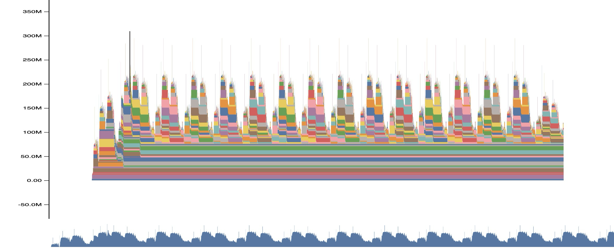
But if we enable the cuDNN autotuner, the peak memory usage can increase significantly.

...
torch.backends.cudnn.benchmark = True
torch.backends.cudnn.deterministic = False
...

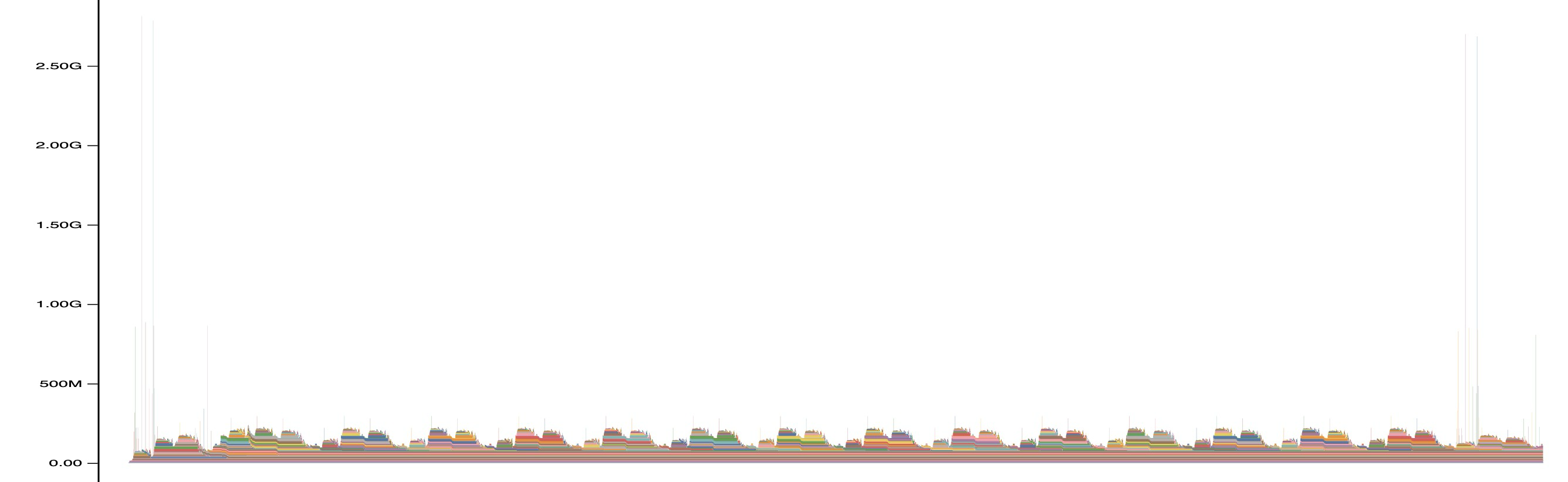
Understanding cuDNN Workspace Spikes

The large memory spikes visible in profiling snapshots (like the 2.5 GiB block in image2.png) originate from cuDNN's algorithm search process during torch.backends.cudnn.benchmark = True.

What happens during the spike:

1. Algorithm search: cuDNN tests multiple convolution algorithms (FFT, Winograd, etc.) to find the fastest one
2. Concurrent workspaces: Each candidate algorithm requests its own workspace buffer (hundreds of MiB to several GiB)
3. Brief coexistence: All workspaces exist simultaneously during the search, creating the large allocation spike
4. Cleanup: Once the best algorithm is selected, workspaces are freed immediately

Key characteristics:

• One-time cost: Same input shapes won't be re-benchmarked in subsequent iterations
• Shape-dependent: New input shapes trigger new searches and potential spikes
• Transient: Memory is freed immediately after algorithm selection
• Invisible in steady-state: Only affects initial iterations or when new shapes appear

References

• Visualize and understand GPU memory in PyTorch ⧉
• A comprehensive guide to memory usage in PyTorch ⧉
• PyTorch memory profiling ⧉
• torch_cuda_memory ⧉
• How to calculate the GPU memory that a model uses ⧉
• Accumulating model output blows up CUDA memory ⧉

2025-12-302026-02-10